Tutorial - Subtomogram averaging with EMAN plugin for Scipion
Table of Contents
List of Abbreviations
STA: subtomogram averaging.
PPPT: per-particle per-tilt.
TS: tilt series.
CTF: contrast transfer function.
Introduction
This tutorial illustrates how to carry out a subtomogram averaging (STA) with a per-particle per-tilt (PPPT) approach using EMAN plugin for Scipion combined with others, listed below for each step:
Import the tilt series (TS) - scipion-em-tomo
Contrast transfer function (CTF) estimation - scipion-em-imod
TS alignment and tomogram reconstruction - scipion-em-emantomo
Import the 3D coordinates - scipion-em-tomo
Generate the initial model - scipion-em-emantomo
Subtomograms refinement - scipion-em-emantomo
The dataset
The dataset used for this tutorial is a subset of EMPIAR-10064, concretely the TS named mixedCTEM_tomo4.mrc (whose details can be found separately in EMD-3420). The dataset also includes:
The estimated CTF, carried out with scipion-em-gctf and converted with Scipion into IMOD CTF format to import it using the corresponding protocol from the plugin scipion-em-imod.
A subset of 200 particles picked with crYOLO inside Scipion (protocol from the plugin scipion-em-sphire).
To download the dataset, simply execute in a terminal the following command:
scipion3 testdata --download emantomo_tutorial_ribo
The dataset will be downloaded to SCIPION_HOME/data/tests.
Associated resources
Here you can find resources associated with this content, like videos or presentations used in courses and other documentation pages:
Preparing the project
First of all, open a terminal and execute the command
scipion3
to run Scipion. After that:
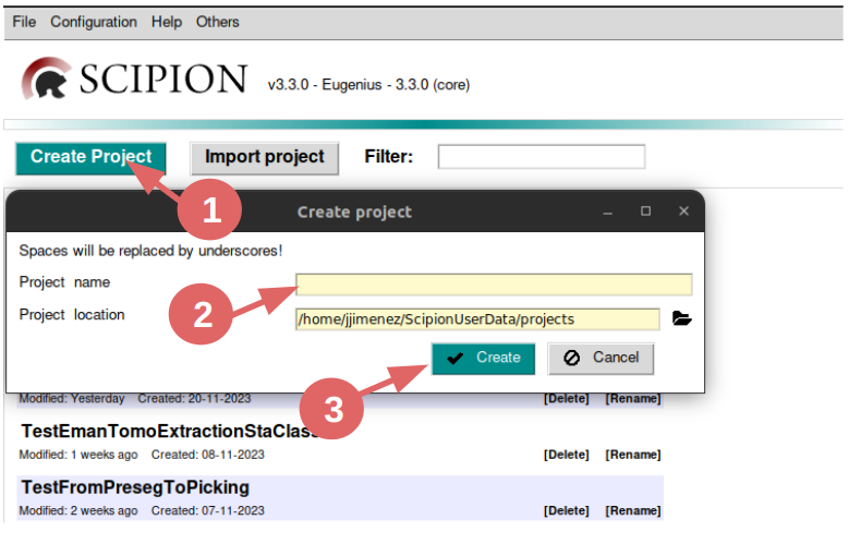
Click on button “Create Project”.
Write a name for it. We’ll name it Day_3_emantomo_sta.
Click on button “Create”.
Note: if starting a project from scratch, the protocols can be located on the left panel of the project interface or directly search via ctrl + f and typing the keywords that may represent what it is desired to be found, like a plugin name, a protocol name, an action, etc.
In our case, we are going to use a Scipion template that contains the the workflow that will be followed in this tutorial customized with the corresponding parameters for each protocol. Nevertheless, the tutorial is described assuming an approach of type “project from scratch”.
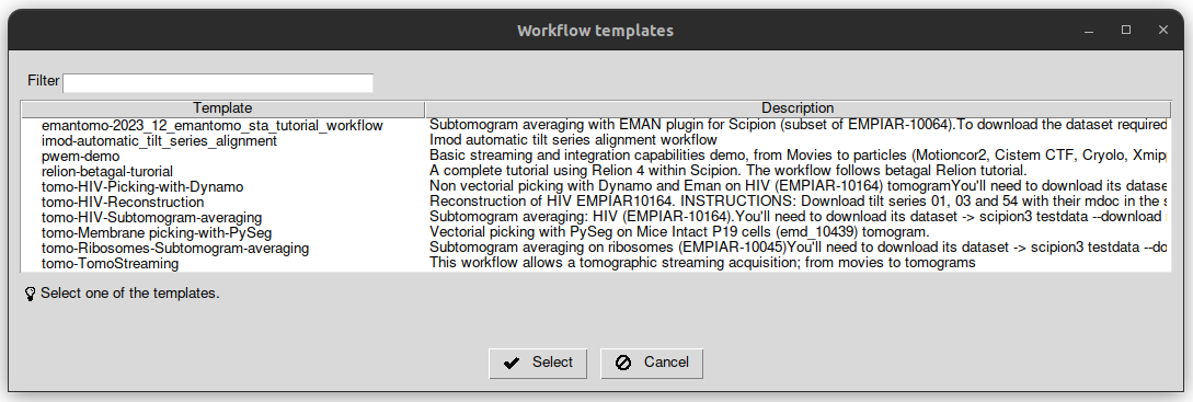
To load the template, clock on the menu named “Others” and then “Import workflow template” on the top left of the project window. After that, a list of the available templates will be displayed. Locate the one named “2023_12_emantomo_sta_tutorial_workflow”, double-click on it or select it and click on the button named “Select”.
This will generate another window, that is used to specify some parameters required by the workflow, normally the file paths. In this case, there is only one, which is the default path of the tutorial dataset downloaded before. Thus, it is not necessary to edit it.
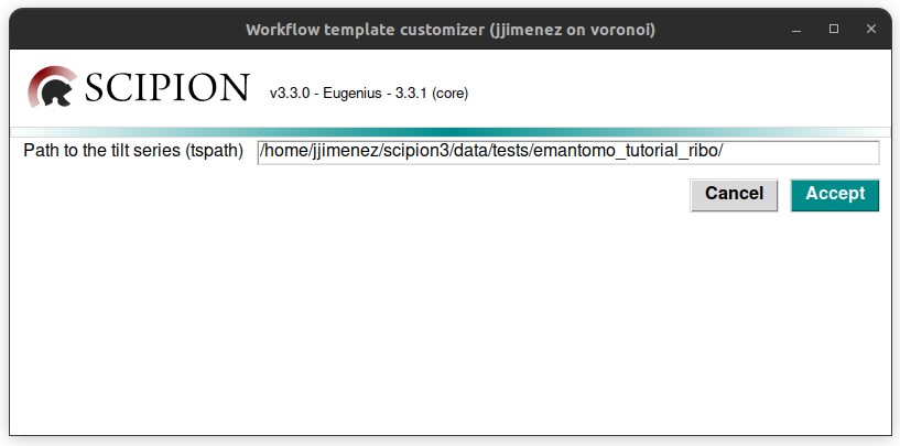
Click on the button “Accept”, and the project graph will be automatically generated, as can be observed in the figure below:
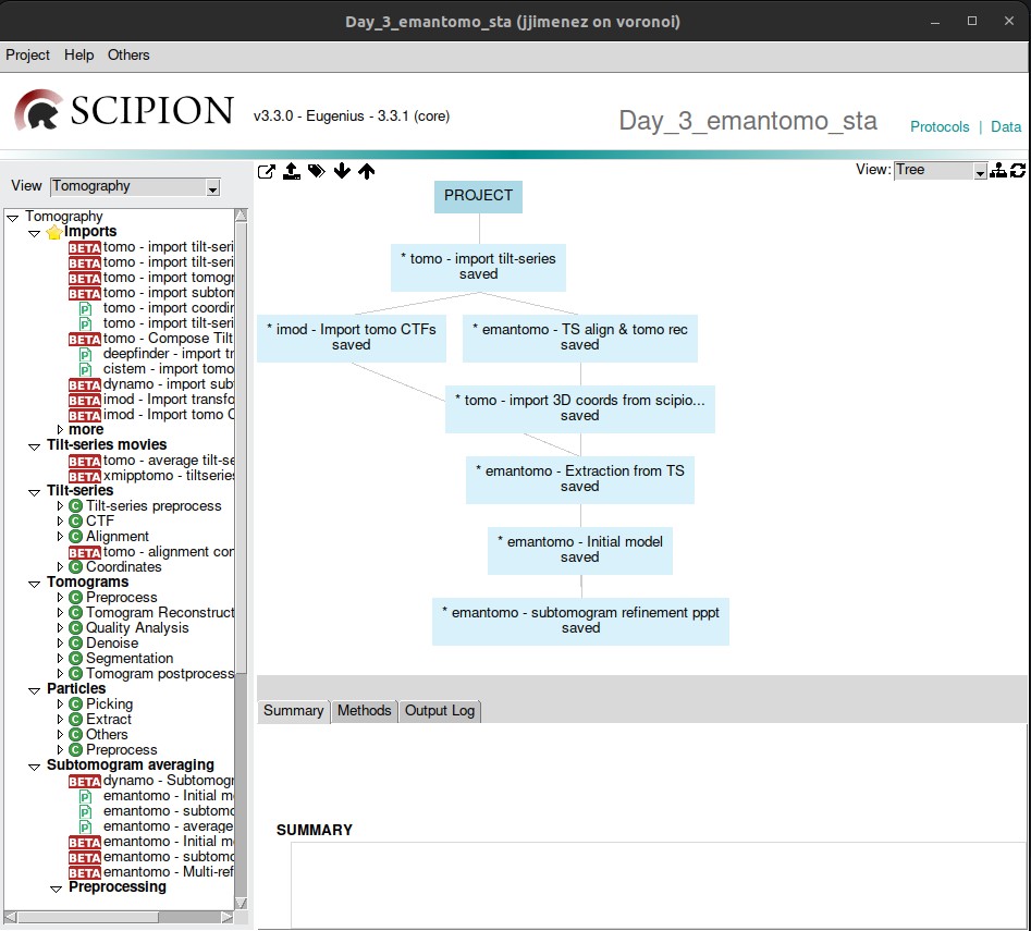
To display the corresponding form of each protocol, simply double-click on it.
Importing the TS
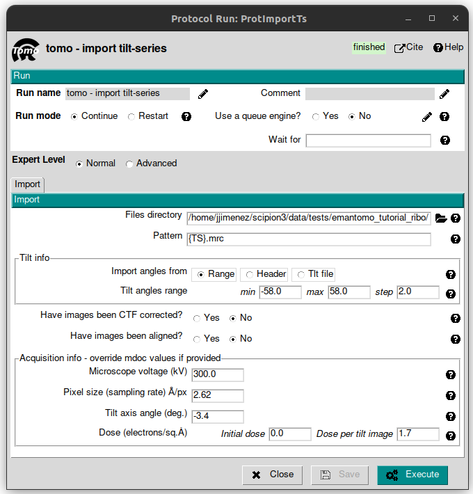
Let’s begin importing the TS. This is the entry point to Scipion, in which external data files are represented as Scipion objects, that is a common representation of the data used to make all the different packages speak to each other. To do that, simply look for a protocol named “tomo - import tilt-series” and click on it. On the tab “Import”, fill the following parameters with the corresponding values listed below:
Files directory: SCIPION_HOME/data/tests/emantomo_tutorial_ribo
Pattern: {TS}.mrc
Tilt angles range: from -58 to 58 with a step of 2
Micorscope voltage (kV): 300
Pixel size (sampling rate) Å/px: 2.62
Tilt axis angle (deg.): -3.4
Dose (electrons/sq.Å) -> Dose per tilt image: 1.7
Leave the rest of the parameters with the default values and click on “Execute” button.
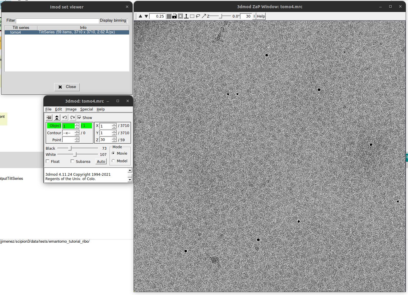
The imported data can be now visualized by clinking on button “Analyze Results”, located on the top right corner of the bottom panel. This will generate an auxiliary window which will list the TS contained in the set imported. In our case, there is only one TS. To open it with IMOD viewer 3dmod (integrated as part of plugin scipion-em-imod), simply double click on it.
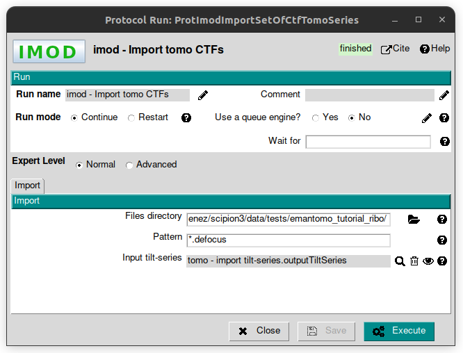
Importing the CTF
In this step, we are going to use the protocol called “imod - Import tomo CTFs” from plugin scipion-em-imod. Once the protocol form is on the screen, fill the following parameters with the values listed below:
Files directory: SCIPION_HOME/data/tests/emantomo_tutorial_ribo
Patterns: *.defocus
Input tilt-series: to get the pointer to the TS previously imported, click on the magnifier icon. This action will open an auxiliary window which will lists the existing objects of the same type as expected.
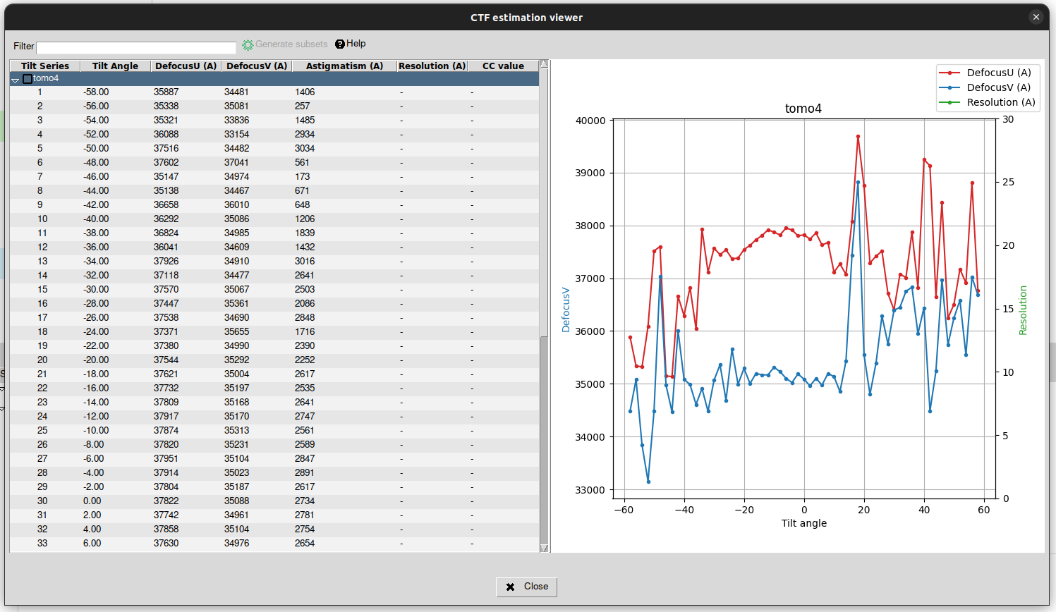
Again, the results can be displayed by clicking on the “Analyze Results” button. The default viewer in this case is the CTF estimation viewer contained in plugin scipion-em-tomo, that looks like as shown in the figure below:
TS alignment and tomogram reconstruction
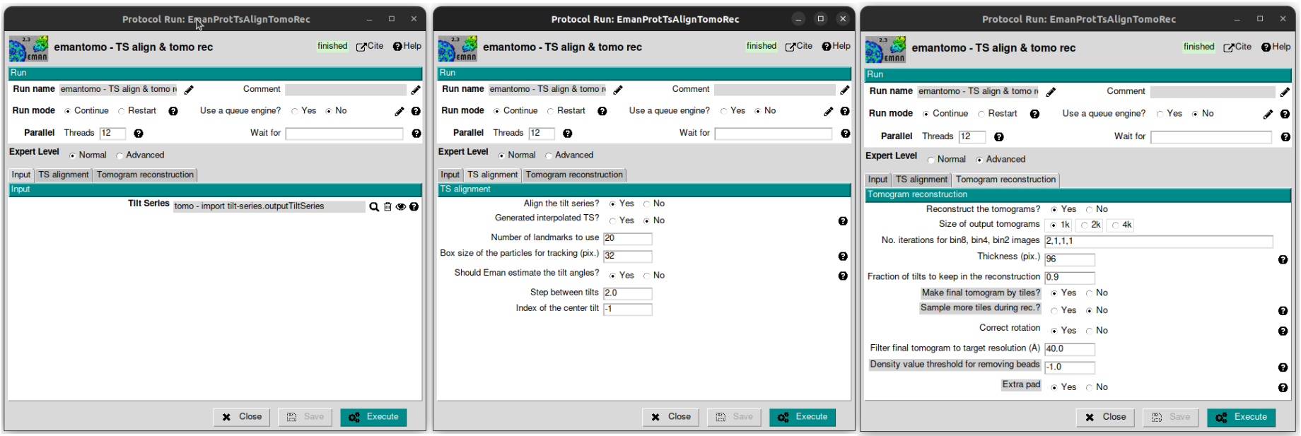
Let’s open the protocol named “emantomo TS align & tomo rec” from plugin scipion-em-emantomo. Fill it with the following values:
Parallel –> Threads: 12
Tab Input:
Tilt Series: select the corresponding object using the magnifier icon.
Tab TS alignment:
Leave all the parameters with the default values.
Tab Tomogram reconstruction:
Expert level: Advanced
Thickness (pix.): 96
Correct rotation: Yes
Extra pad: Yes
Leave the rest of the parameters with the default values.
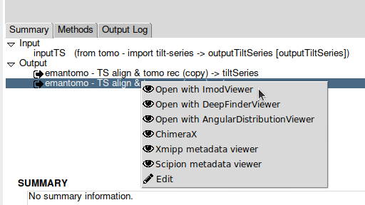
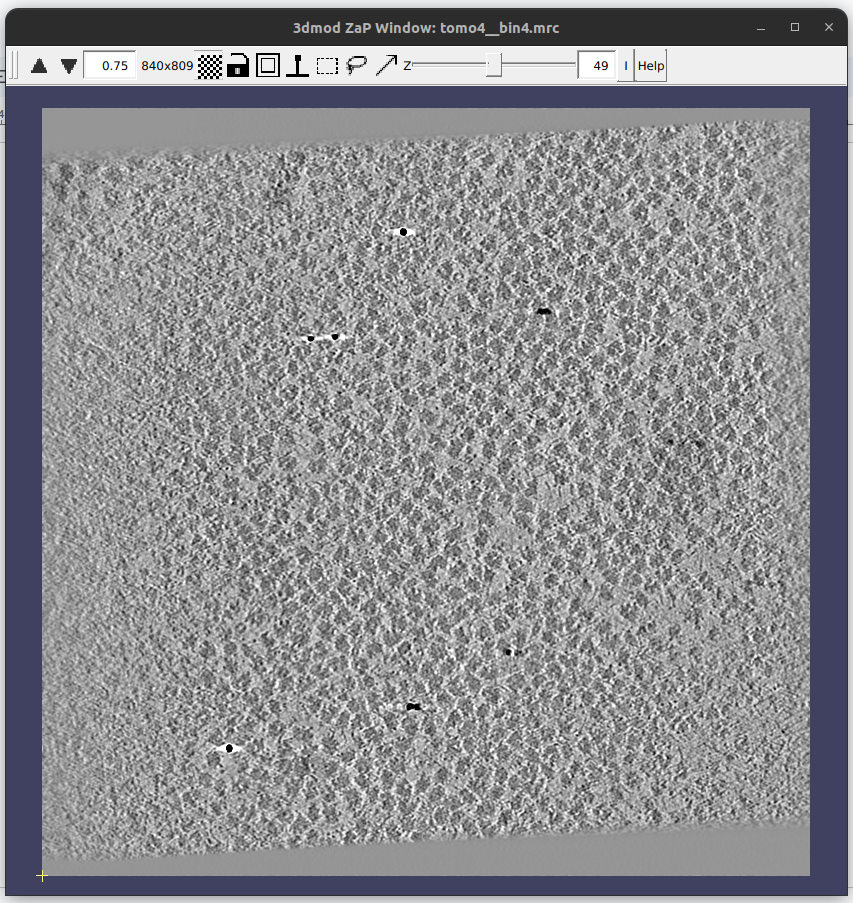
Let’s have a look at the tomogram reconstructed. To do that, right-click on the tomograms output listed in the summary tab located on the lower half of the project main window and select “Open with ImodViewer”.
Then, a new window containing the list of tomograms (only one in this case) will be generated. Double click on it to launch the selected viewer with that data. It should look like the figure below:
Importing the 3D coordinates
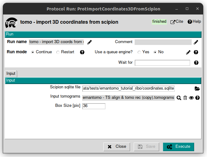
To import the provided coordinates, open the protocol named “tomo - import 3D coords from scipion” from the plugin scipion-em-tomo. Fill the following parameters with these values:
Scipion sqlite file: SCIPION_HOME/data/tests/coordinates.sqlite
Input tomogras: select the corresponding object from the list displayed after having clicked on the magnifier icon.
Box size [pix]: 36
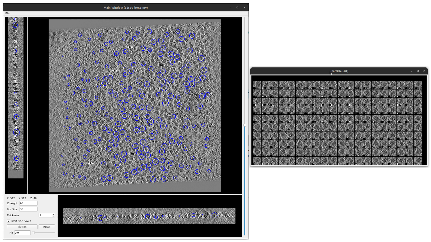
Let’s use tho do that, right-click on the output object listed in the project’s summary panel, and select “Open with Eman”:
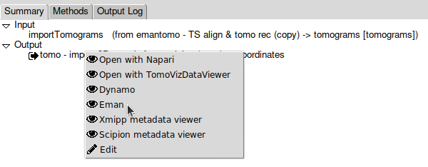
On the list displayed, double click on the set of coordinates listed. They should look like this:
Note:
Once the viewer is closed, a new window will appear to ask if you want to save the protocol output. It is because some viewers, like this one, allow the user to add or remove elements (coordinates in this case). In nothing was changed or you don’t want to save the changes done from the viewer, simply select “No”.
Particle extraction from the TS
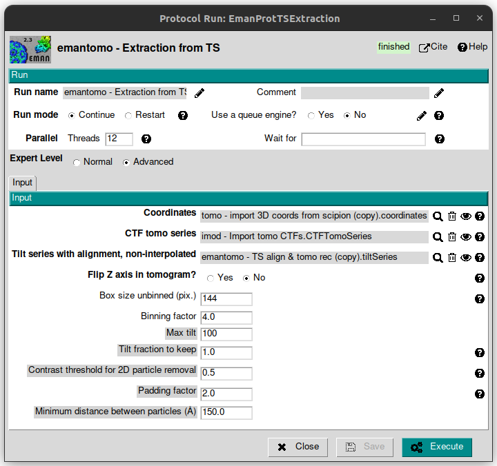
This protocol uses the CTF estimation, TS alignment and coordinates data to go back to the TS and crop an image for each particle for each tilt image (PPPT approach) and the uses them to reconstruct a 3d particle. To carry out this step, let’s open the protocol “emantomo - Extraction from TS” from plugin scipion-em-emantomo and fill the following parameters with the values listed below:
Threads: 12
Expert Level: Advanced
Coordinates: select the corresponding object clicking on the magnifier button.
CTF tomo series: select the corresponding object clicking on the magnifier button.
Tilt series with alignment, non-interpolated: clicking on the magnifier icon will display a list of two available objects, which correspond to the imported TS and the TS with alignment data from the previous step. This is the one that must be selected, that should appear the first in the list.
Flip Z axis in tomogram? No
Box size unbinned (pix.): 144
Binning factor: 4 (thus, the generated particles box size will be 144 / 4 = 36 pix.).
Contrast threshold for 2D particle removal: 0.5 (remove gold beads).
Minimum distance between particles (Å): 150 (as 300Å is the highest ribosome size value from its size ranges).
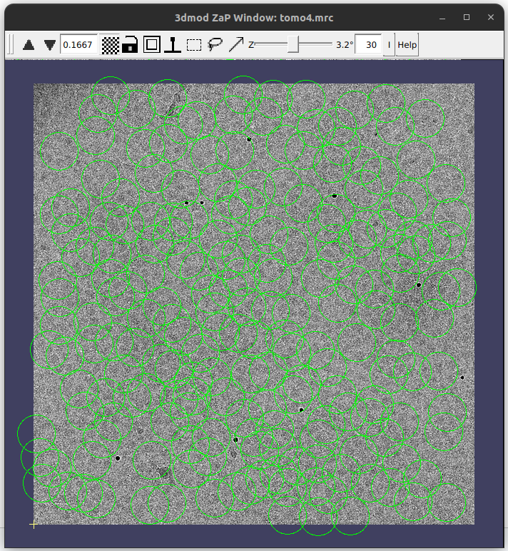
The best way to check if the particles were correctly referred to the TS is to display with the IMOD viewer the generated result called projected2DCoordinates. It will show the extracted particles over the TS, as can be observed in the figure below:
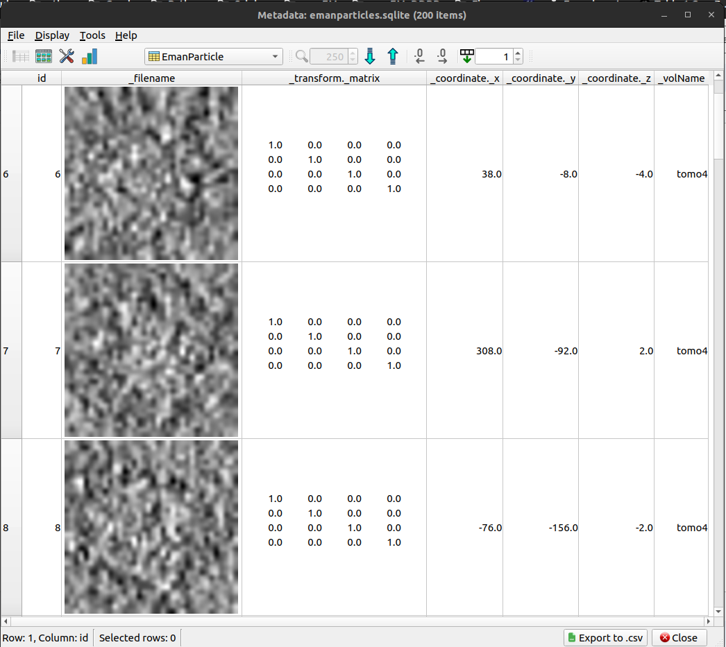
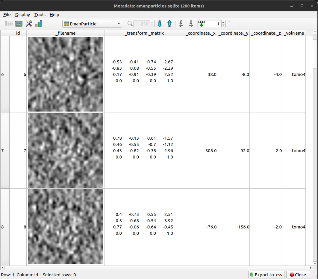
Also, the generated subtomograms can also be displayed. Let’s select in this case, the Scipion metadata viewer. It should look like as shown in the figure below:
Generate the initial volume
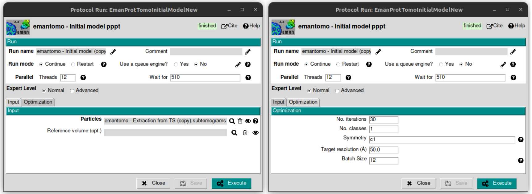
Once we have the particles extracted, it’s time to calculate an initial volume with them. To do that, open the protocol named “emantomo - Initial model pppt” rom plugin scipion-em-emantomo and fill the following as listed below:
Threads: 12
Tab Input
Particles: select the corresponding object by clicking on the magnifier icon.
Reference volume (opt.): leave this empty.
Tab Optimization
No. iterations: 30
Leave the rest of the parameters with the default values.
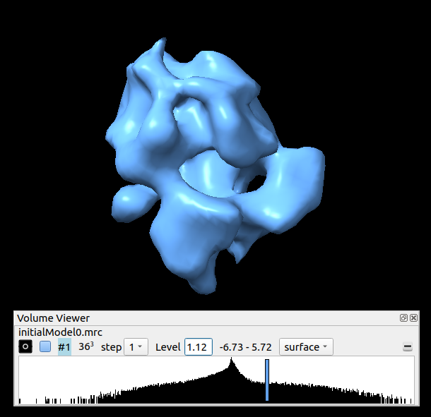
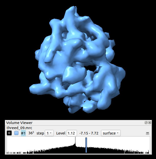
The generated output will be a set of averages, one for each class specified. In this case there will be only one as the number of classes introduced in the protocol form was 1. Sometimes it can be very useful to specify more than one class even if there is only one class, and then select the best one, as sometimes the convergence is not reached and the result is not good. On the other hand, the higher number of classes introduced, the longer it will take the protocol to finish. Said that, let’s open our initial model, in this case with Chimera. It should look like as in the figure below:
Subtomogram refinement
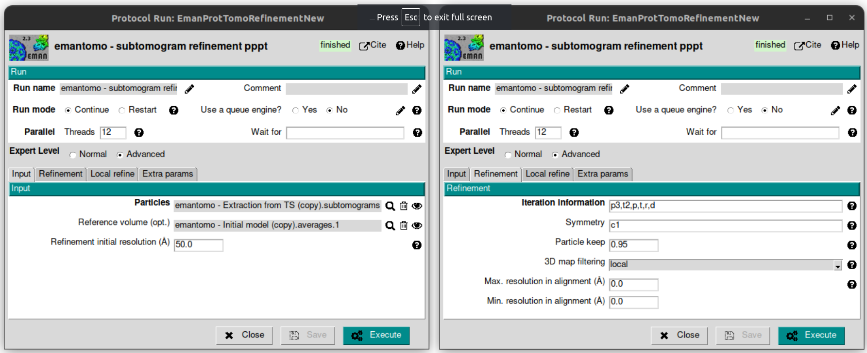
Finally, let’s use the generated initial model and the extracted subtomograms to generate a refined average. To do that, let’s open the protocol “emantomo - subtomogram refinement pppt” from the plugin scipion-em-emantomo, and fill the following parameters with the values specified below:
Threads: 12
Tab Input:
Particles: use the magnifier icon and select the particles extracted from the TS.
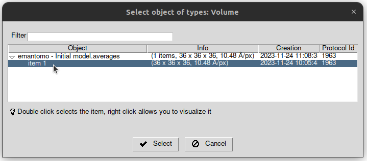
Reference volume (opt.): again, click on the magnifier icon and select the item 1 from the set of averages generated in the previous protocol.
Tab Refinement:
3D map filtering: local
Leave the rest of the parameters with the default values.
Regarding the parameter “Iteration information” in the tab “Refinement”, it admits combinations of four types of refinements, which are:
p: 3d particle translation-rotation.
t: subtilt translation.
r: subtilt translation-rotation.
d: subtilt defocus.
The default value is p,p,p,t,p,p,t,r,d. It can be compacted using the corresponding character followed by the desired number of iterations of that type, e. g., p3 = p,p,p.
This protocol generates 3 outputs, that are:
The refined average.
The refined subtomograms.
The FSC curves.
Let’s display it:
The refined average, using Chimera:
The refined subtomograms, displayed with Scipion metadata vierwer:
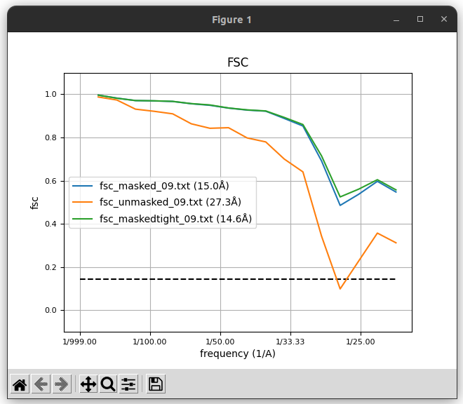
The FSC curves, displayed with Scipion FSC viewer.
Full dataset results
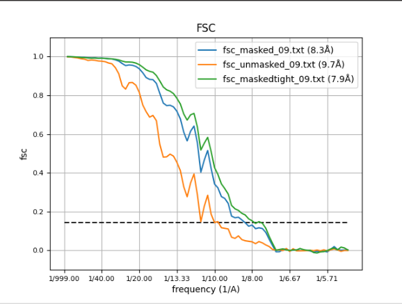
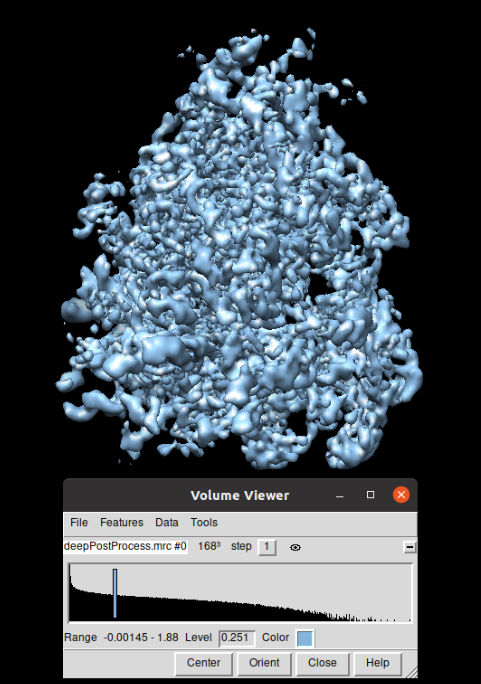
The same workflow was carried out with all the TS (mixedCTEM ones) that compose the dataset EMPIAR-10064. The corresponding refinement result (displayed with Chimera) at bin 1, together with the FSC curves are shown below:
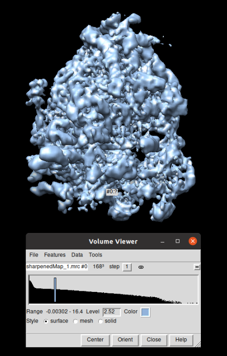
The volume obtained was sharpened using the protocol localdeblur sharpening from the plugin scipion-em-xmipp. The resulting volume can be observed in the figure below, displayed again with Chimera:
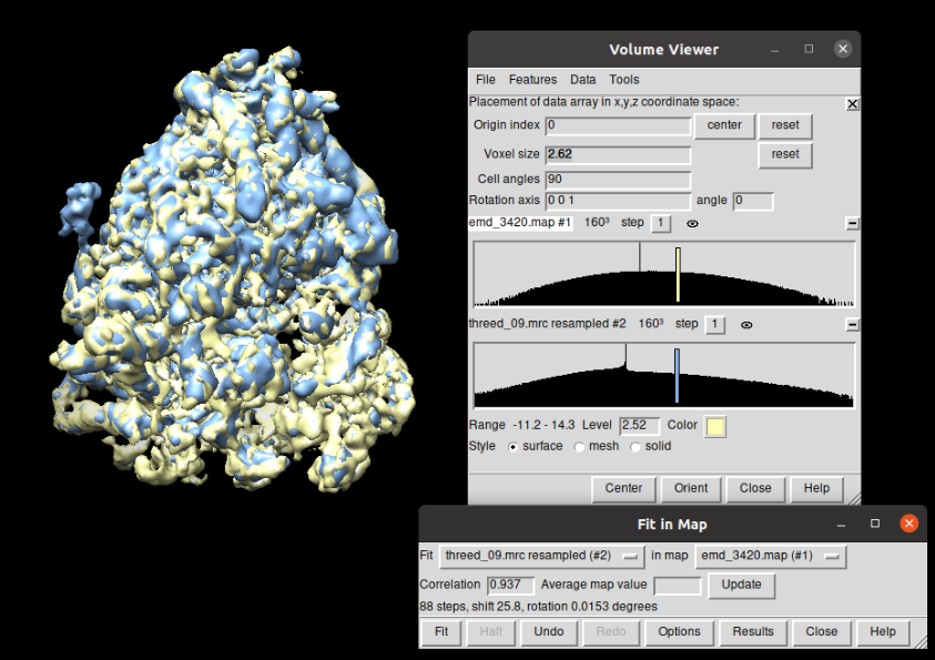
Compared to the corresponding EMD dataset (EMD-3420), the resolution it can be observed that the resolution achieved with the workflow proposed is higher that the reported in EMD (8.3Å vs 11.2Å). The figure below shows the superposition ob both structures (EMD in yellow and the one obtained in blue) displayed with Chimera. It can be observed that the correlation between both structures is 93.7% (Thanks to Patricia Losana from BCU CNB-CSIC for the help with Chimera).
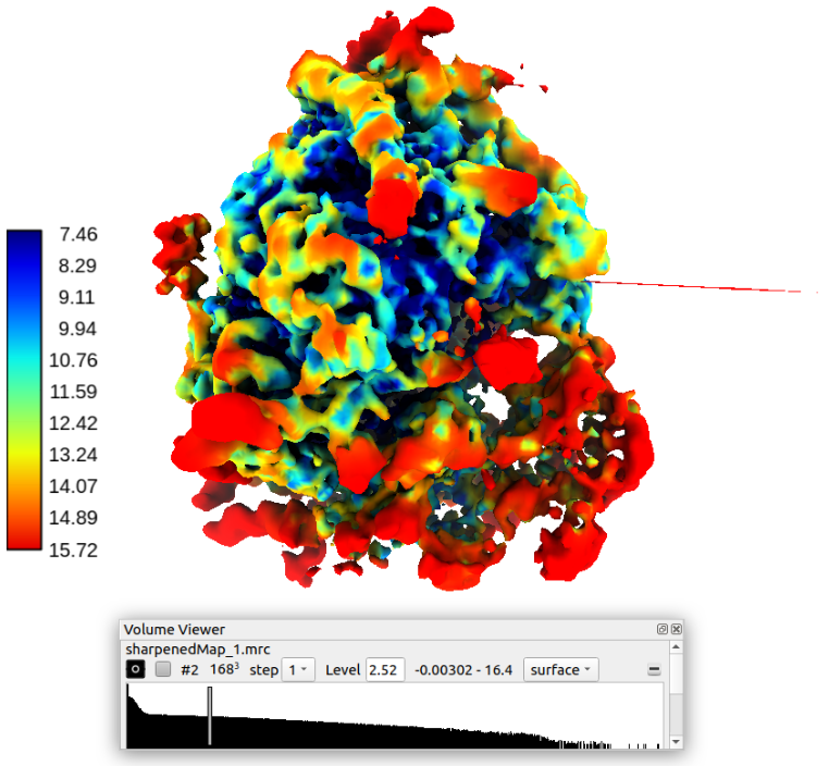
Finally, the local resolution was estimated using the protocol MonoRes from the plugin scipion-em-xmipp. The following figure shows the local resolution map over the sharpened structure displayed with Chimera (Thanks to José Luis Vilas from BCU CNB-CSIC for the help with the local resolution and sharpening).