Flexibility Hub: Advanced guide

This tutorial is structured around a workflow defined with experimental data. The data for this tutorial can be downloaded with scipion3 testdata --download FlexHub_Tutorials.

Note that the workflow tutorial focuses mostly on the way flexibility information can be analysed from CryoEM particle data. To that end, the different algorithms will be used to exemplify the workflow.

Apart from the particle workflow proposed, there exists other possibilities inside the Flexbility Hub to extract information from CryoEM maps and structural models as well. If you are interested on knowing more about all the functionalities in the Flexibility Hub, we propose reading the specific Plugin tutorials provided above.

Workflow tutorial

Some comments on the data to be used

In this tutorial, we will use the EMPIAR-10028 dataset. However, we will be working with a post-processed version of the dataset where angular information has been gone through a consensus step to improve its accuracy. We strongly recommend doing consensus analysis before defining a flexibility workflow, as the conformational landscapes estimation depend strongly on the aligment of the particles. The modified dataset includes:

• Particles: we will work with around 50K particles with (consensuated) angular information and CTF.

• Volume data: map reconstructed from the particles (needed by some of the algorithms to be used during the workflow)

• Structural model: to be used to analyze conformational changes at atomic level.

We should note that CTF information is usually mandatory for most flexibility algorithms. However, in some cases it might be possible to use corrected particles as well. We will comment on these possibilities during the tutorial.

Where to find Flexibility Hub protocols?

Flexibility Hub related protocols have been grouped in a new View tab in the Scipion GUI called Flexibility Hub. In addition, it is possible to use the key Ctrl+F to open a protocol search dialog.

1. Importing the data in Scipion

The first step in our workflow is to import our particles, volumes, and structural models in Scipion.

Here we provide a tutorial for importing data inside Scipion. Below it is also provided the filled form to import our particles, which also includes the sampling rate that will be needed to import the map and mask.

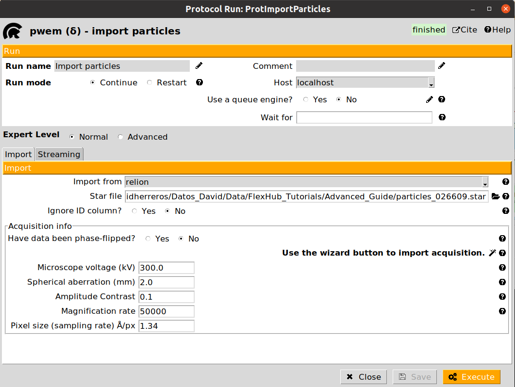
Once all the data has been imported, we are ready to start the flexibility analysis. Note that in a real project, the input data to the Flexibility Hub (particles, maps, models…) might come from different sources (imports, refinements, consensus…).

2. Zernike3Deep landscape estimation

Flexutils includes several Zernike3D programs able to estimate conformational landscapes from CryoEM particles. Among them, generally the best possible choice to start any analysis is the Zernike3Deep algorithm.

The Zernike3Deep method is a semi-classical neural network able to learn to produce meaningful Zernike3D coefficients compatible with the mathematical basis description. Therefore, it uses our own knowledge during the learning process, producing a results that is no longer a black box.

The Zernike3Deep pipeline is divided into two different protocols:

• angular align - Zernike3Deep: Protocol responsible of training the Zernike3Deep network based on a set of input particles. In addition, it will also infer Zernike3D coefficients for those same particles.

• predict - Zernike3Deep: Protocol to infer new Zernike3D coefficients from a previously trained Zernike3Deep network and a new set of particles.

In our workflow, we will exemplify the use of both protocols. Let’s start with the training of the Zernike3Deep network. An example of the form is provided below:

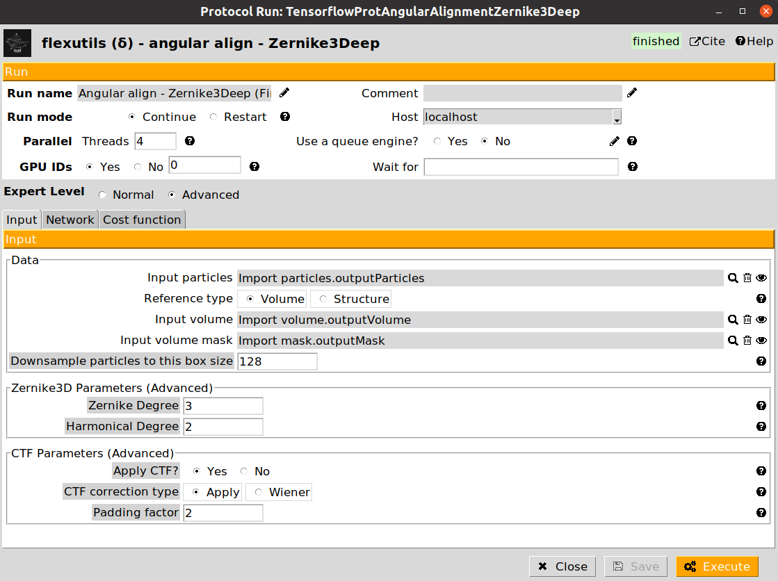
The form is subdivided into three different tabs (Input, Network, and Cost function). For this workflow, we provide below the parameters to be filled up:

• Input section

  • Input particles: Particles previously imported in the Scipion project

  • Reference type: Select Volume for this step

  • Input volume: The map previously imported in the Scipion project

  • Input mask: The mask previously imported in the Scipion project

• Network section

  • Number of training epochs: Increase it to 50 since we have a low number of particles

• Cost function section (leave as default)

Once filled up, you can click on the Execute button to start tranining the Zernike3Deep network. Once it finishes, you should see an output of type SetOfParticlesFlex on the Summary Scipion tab. The output particles will include all the information stored in the input ones, as well as the conformational landscape information estimated by the network.

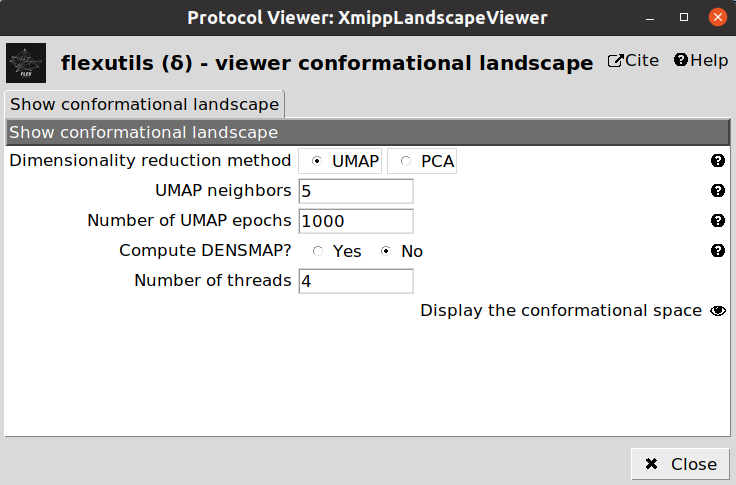
One way to check the initial shape of our landscape is to use the Flexutils visualization tools. At the current step, we can visualize the estimated landscape by clicking on . You should see a form like this:

3. CryoDRGN landscape estimation

CryoDRGN is a heterogeneity algorithm able to estimate compositional and continuous variability from a CryoEM particle dataset.

To that end, CryoDRGN relies on a neural network designed to learn how to reconstruct CryoEM maps from particles, given the CTF and the angular information previously estimated. In addition, the network is able to account for the conformational variability thanks to a latent space that captures the conformational landscape representation, allowing to perform heterogeneous reconstructions.

The CryoDRGN implementation is divided into two different steps, represented by two different protocols in the Flexibility Hub:

• Preprocess step: Preparation of the particle dataset so it can be input in the neural network. The output of this step is a new set of particle containing all the information needed by the training step.

• Training VAE step: Training of the CryoDRGN neural network with a set of particle previously prepared with a CryoDRGN preprocessed protocol. The output of this step is a set of particles contanining the conformational landscape estimated. In addition, a set of volumes is also registered, which provides an initial inspection of several conformational states learned by the network.

We will start the CryoDRGN pipeline by executing the preprocess step to prepare our particles. An example of the form is provided below:

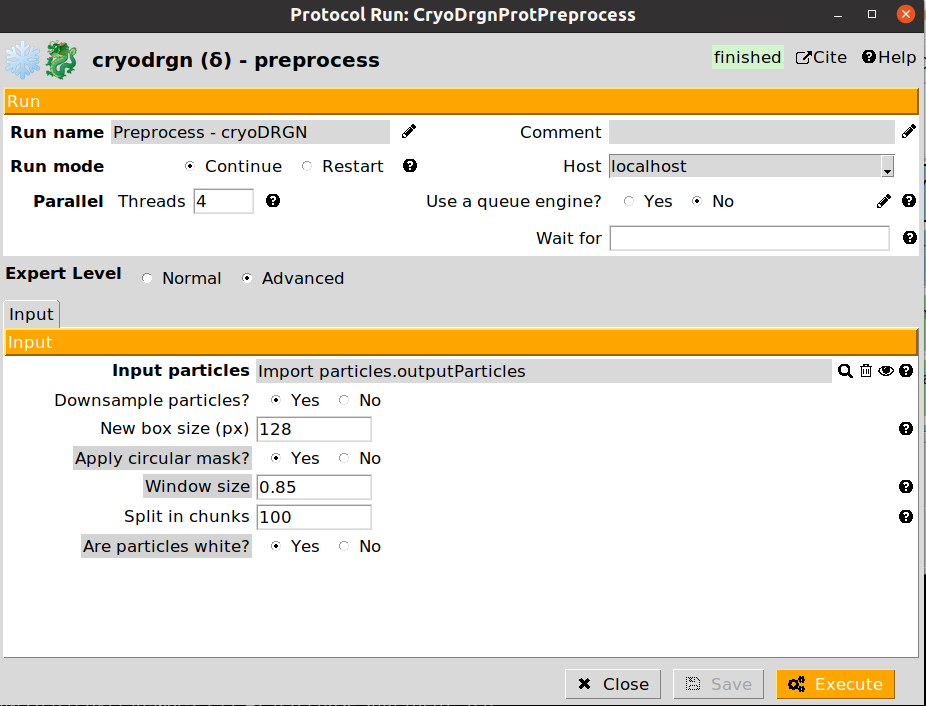
The preprocessing step allows to downsample the particles to a smaller boxsize. This is usually desirable in order to improve performance, and avoid/solve possible GPU memory errors during the training step. However, it is important to note that the maps decoded by the network will be restricted to the downsampled boxsize. Therefore, it is important to determine the minimum resolution needed to analyze a given conformational change, and downsample the particles accordingly.

The parameter Split in chunks controls the number of particles that will be process at a time (similar to a batch size). If you experience any memory issues during the preprocessing, setting a smaller value might solve the issue.

Once the particle preparation step is done, we can start training the CryoDRGN neural network. The form of the Training VAE step is provided below:

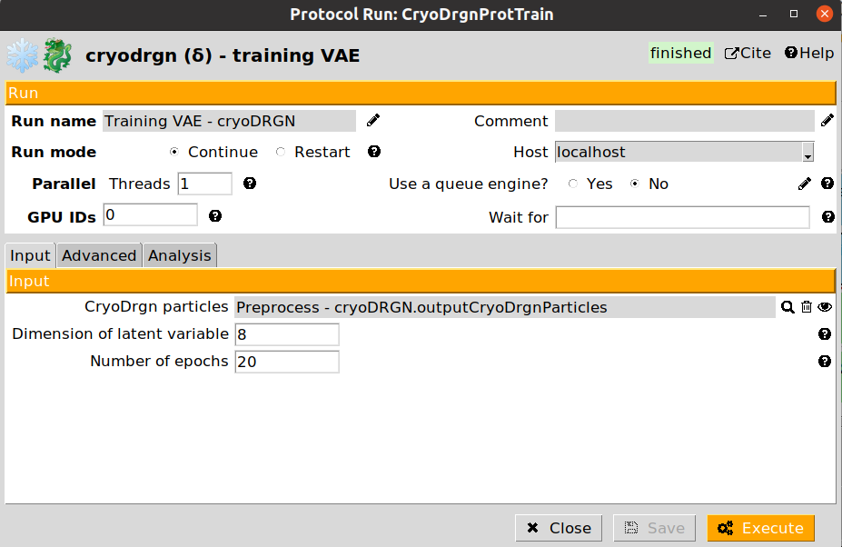
The CryoDRGN training protocol form is split into three different sections:

• Input section

  • Cryodrgn particles: Particles generated by a CryoDRGN preprocess protocol

  • Dimension of latent variable: Latent space dimensions. The higher the dimensions, the larger the freedom CryoDRGN will have to approximate conformational states (large values may induce overfitting). It is recommended to set a value between 8 and 10.

  • Number of epochs: Number of training epochs. Depending on the downsampling applied to the particles, it might be needed to increase the value provided by default.

• Advanced section

  • This section allows to fine tune the network architecture. In general, it might not be needed to modify the default values. In addition, it provides a way to pass to CryoDRGN any parameter not included in the protocol form.

• Analysis section

  • This section will determine the number of maps to be decoded after training the CryoDRGN network, which might be useful to have an initial inspection of the estimated states.

Once filled up, you can click on the Execute button to start tranining the Zernike3Deep network. Once it finishes, you should see an output of type SetOfParticlesFlex on the Summary Scipion tab. The output particles will include all the information stored in the input ones, as well as the conformational landscape information estimated by the network.

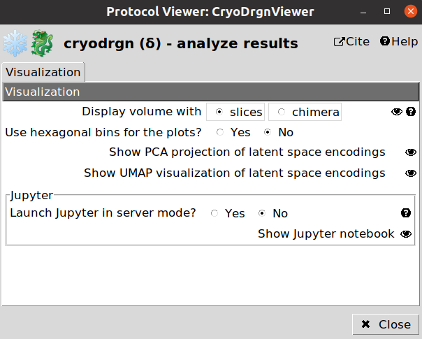
One way to check the initial shape of our landscape is to use the CryoDRGN visualization tools. At the current step, we can visualize the estimated landscape by clicking on . You should see a form like this:

4. HetSIREN landscape estimation

HetSIREN is an algorithm able to estimate continuous and compositional heterogeneity from CryoEM particles.

It is based on a neural network able to learn how to perform heterogeneous reconstruction in real space. Therefore, it is possible to focus the analysis on different map regions, learn reconstruction from scratch, or use a reference map as an initial guess.

In addition, HetSIREN has been designed so it can learn to reconstruct, denoise, and sharp simultaneously, leading more accurate representations of the different estimated states.

The HetSIREN pipeline is divided into two different protocols:

• angular align - HetSIREN: Protocol responsible of training the HetSIREN network based on a set of input particles. In addition, it will also infer the HetSIREN latent space for those same particles.

• predict - HetSIREN: Protocol to infer new HetSIREN latent spaces from a previously trained HetSIREN network and a new set of particles.

In our workflow, we will exemplify the use of both protocols. Let’s start with the training of the HetSIREN network. An example of the form is provided below:

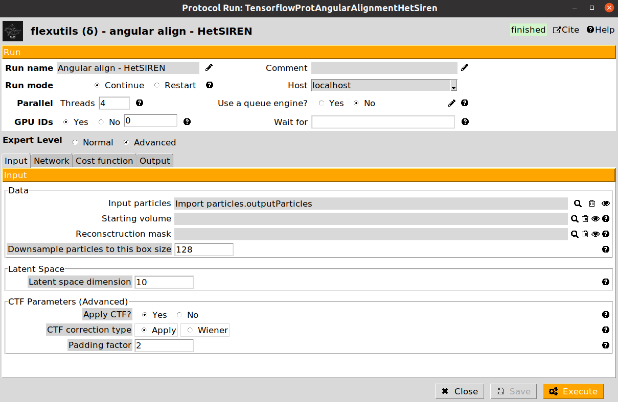
The form is subdivided into three different tabs (Input, Network, and Cost function). For this workflow, we provide below the parameters to be filled up:

• Input section

  • Input particles: Particles previously imported in the Scipion project

  • Leave remaining parameters as default

• Network section (leave as default)

• Cost function section (leave as default)

Once filled up, you can click on the Execute button to start tranining the HetSIREN network. Once it finishes, you should see an output of type SetOfParticlesFlex on the Summary Scipion tab. The output particles will include all the information stored in the input ones, as well as the conformational landscape information estimated by the network.

Similarly to the previous sections, it is possible to check the initial shape of our landscape is to use the Flexutils visualization tools. At the current step, we can visualize the estimated landscape by clicking on . You should see a form like this:

5. Flexibility consensus

At this point, we have perform three independent executions of different algorithms and obtained their corresponding conformational landscapes. The next question we should answer is to decide how confident we really are on the different estimations we have obtained.

Due to the intrinsic complexity of conformational landscapes, it is difficult to do a confidence analysis of the results by hand. Thus, the easiest way to analyze the conformational landscapes’ agreement is to do a flexibility consensus.

Flexutils include a new flexibility consensus pipeline able to determine a consistency measurement of each particle based on different estimations of its conformational landscape. In this way, it is possible to keep only those particles that have been assigned a similar conformational state, increasing the reliability of the landscapes we have estimated.

The flexibility consensus pipeline is divided into two different step:

• Train - FlexConsensus: this step will train the flexibility consensus network based on several landscape estimations.

• Interactive consensus - FlexConsensus: this step allows to interactively select the particles to be kept based on a trained consensus network.

Let’s start by training our flexibility consensus network with the three landscape estimation obtained from the Zernike3Deep, CryoDRGN, and HetSIREN algorithms. Below we provide and example of the filled form of the protocol:

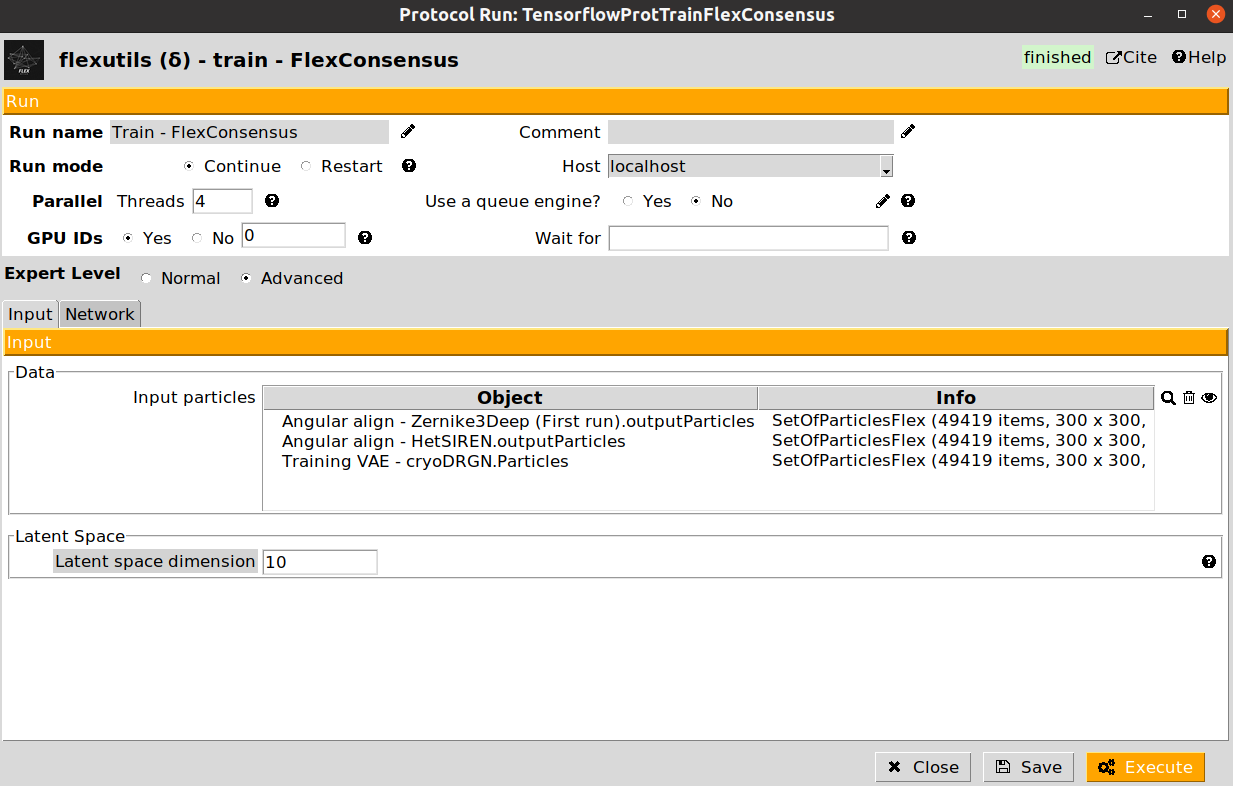
The training protocol will not register any output in Scipion once it finishes. Instead, it will generate all the information needed to interactively select the particles we are interested in during the interactive step.

Once the training has finished, we can execute the interactive particle selection step. The form of the protocol is provided below:

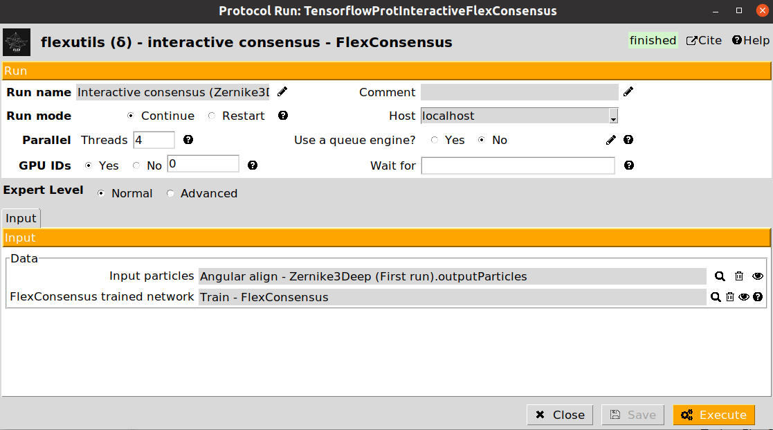
In the form, we can provide a set of particles (with landscape) generated from any of the programs we have input in the consensus training step. For example, if we input particles coming from a Zernike3Deep estimation, during the interactive consensus we will get a more consistent set of particles with Zernike3D information. This gives more freedom to the analysis, as we are not losing any kind of information during the consensus step.

The interactive consensus protocol will estimate the consistency measurements for the input particles provided based on a trained flexibility consensus network. Once the protocol has finished, we can click on to start the interactive selection tool. This will open the following window:

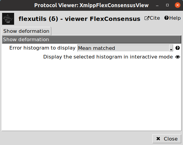
We have two ways of displaying the estimated particle consistency histogram:

• Mean matched: Histogram showing a representation based on the lowest errors estimated during the training step.

• Entropy matched: Histogram showing a representation based on the highest entropy of the errors estimated during the training step.

After opening the interactive tool on any of the previous two modes, we should get something similar to the following image:

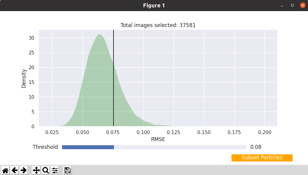
The tool shows the consistency histogram for our particles, and allows to interactive determine a consistency threshold to exclude undesired particles. The title of the histogram plot displays the number of particles that will be kept for the current threshold. By clicking on Subset particles we can generate a new set of particles containing only the most consistent particles for the selected threshold. It is possible to generate as many subsets as desired, as they will be registered independently inside Scipion.

6. Landscape dimensionality reduction

Since the landscape estimated after the consensus step has a large number of dimensions, we need to reduce them to a number that we can handle (usually, 2D or 3D). To that end, we can apply the dimensionality reduction protocol from Flexutils to get a meaningful representation base on different methods.

Currently, the methods included are the following:

• PCA: Dimensionality reduction based on Principal Components Analysis. This linear method is very popular, but the representation obtained is usually not very informative unless states are well separated.

• UMAP: Non-linear dimensionality reduction method. UMAP landscapes are usually more informative than PCA, although in some cases it might lead to some artefactual generated regions.

• DeepElastic: Non-linear dimensionality reduction based on elastic analysis of clusters. it usually gives results in the middle between PCA and UMAP.

Since the dimensionality reduction is fast, we recommend running the three methods, and use the button to check which provides a better representation for a given dataset. Note that the is currently implemented only for 3D spaces.

We provide below some images of the forms filled to run any of the different dimensionality reduction methods for the tutorial dataset:

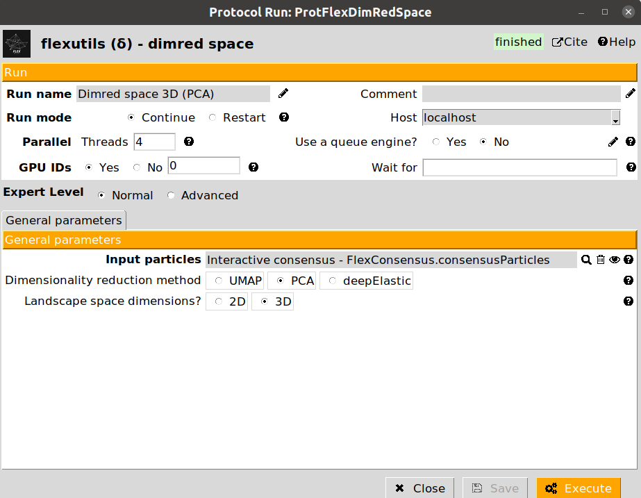
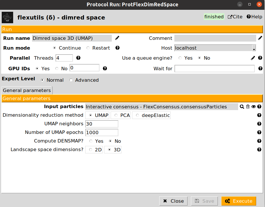
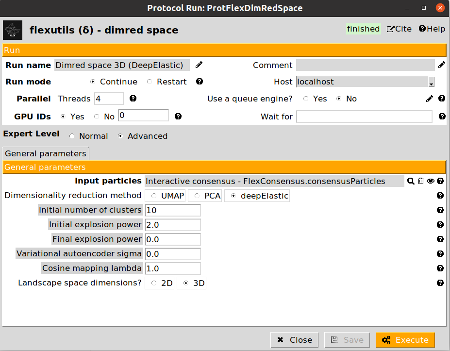
We recommend checking the results obtained with the different methods, as their performance may vary depending on the dataset. For the next sections in the tutorial, we will use the UMAP representation, although the subsequent sections could be replicated with any of the other two other methods.

7. Interactive landscape clustering

Once the consensus landscape has been reduced, it is possible to use the interactive tools implemented in Flexutils to explore the different states found. In our case, we have decided to use the Zernike3Deep landscape estimation to generate the consensus output, although the following analysis could be performed with CryoDRGN and HetSIREN as well.

Flexutils interactive tools has been developed for both, 2D and 3D spaces, and include two different ways to explore the data:

• Cluster space (only for 3D spaces): Interactive clustering of flexibility spaces based on KMeans. The tools provides two visualization windows:

  • Left panel: 3D visualization of the point cloud representing the conformational landscape of the molecule

  • Right panel: Map visualization obtained from a selected cluster

The space can be clustered as many times as needed, based on the number of clusters specified in the corresponding field in the right panel. Once clustered, it is possible to click on any of the cluster representatives (white dots) in the left panel to get a real time representation of the map coming from that specific point. In addition, the viewer provides a shortcut to view the map representatives in ChimeraX for advanced visualization of the conformational states. * Annotate space (for 2D and 3D spaces): Provides and interactive way to explore any region from a given conformational landscape. Therefore, it is possible to click anywhere in the landscape view to get in real time the conformational state corresponding to the selected landscape region. Similarly to the previous tool, there exists a shortcut to ChimeraX for advanced visualization.

Video tutorials explaining the usage of the different tools are available here. We recommend watching these videos at this point before doing your first landscape exploration.

We provide below the filled form of the Cluster space protocol as an example:

In this case, the form only requires as input a set of particles coming from a dimensionality reduction protocol. Since Cluster space is only implemented for 3D spaces, the protocol will validate before executing whether the reduced space stored in the particle set has the appropriate dimensions.

Both, Cluster space and Annotate space protocols will register inside Scipion a set of classes (with flexibility information) based on your saved annotation. The set of classes provides a very convenient way to store the information extracted from the lanscape. By clicking on you will be able to:

• Inspect the set of classes information (representatives, particles associated with each representative, flexibility information…)

• Create a subset of new classes

• Create a subset of representatives (useful to further analyze states from the flexibility information stored)

• Create a subset of particles associated with a given representative (useful to refine a given state)

Let’s extract the representatives of the classes using with button. Thanks to this extraction, it will be possible to further analyze the Zernike3D coefficients to extract the conformational states of the representatives and get more information about the motions suffered by the protein.

8. Applying deformation fields

If we try to open any of the representative volumes extracted from the set of classes generated in the previous step, we will see that all the maps are identical to the reference volume we imported at the beginning of the workflow. Instead, the Zernike3D programs (and other programs estimating motions based on deformation fields) provide several tools to continue analyzing flexibility information, being one of those tools the application of the estimated deformation fields to approximate a new conformational state.

The protocol apply deformation field - Zernike3D is the one responsible for this task. The protocol form will ask for a set of volumes with Zernike3D flexibility information stored. The Zernike3D flexibility information will be used to restore an estimated deformation field to be warped to yield a new state.

In addition, the protocol allows to provide an atomic structure (that should be ideally traced, or at least aligned against the reference map used during the Zernike3D estimations). If provided, it will be possible to get the new state as a structural model instead of as a density map.

By clicking on , it is possible to inspect in different ways the new states (either at map or structural model level). Two of the options provided include seeing a strain or rotation color map computed from the estimated deformation fields. The strain/rotation maps summarize the information about the forces suffered by the protein when transition from the reference state to the new state we have just estimated:

• Strain map: Summarizes the compression/stretching forces

• Rotation map: Summarized the rotational forces

We provide below an example of the strain visualization in ChimeraX:

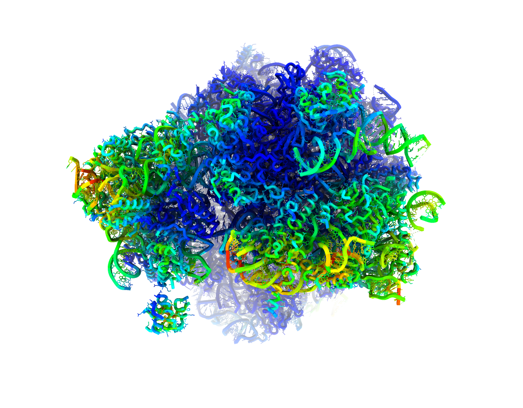
Depending on the provided inputs in the protocol form, the visualization will show either a map or a structural model painted according to the strain/rotation forces acting on each voxel/atom. In the colormap, red colors translates into larger rotational/strain forces while blue colors represent those regions suffering lower forces.

9. Motion statistics

As we saw in Section 7 from this tutorial, the flexible classes obtained after an interactive conformational space clustering and/or annotation will store the 3D conformational states (or the information needed to recover them), and the particles associated with that 3D conformation.

The flexible classes viewer allows extracting any of these two previous information. For example, we can extract the particles associated with on of the selection by clicking on the desired selection and pressing the button.

The extracted particles cna be further analyzed by several means to better understand the heterogeneity they represent. One of the previous possibilities is to visualize the average deformation field computed from the particles, which provide a better understanding of the estimated local motions affecting our macromolecule.

The protocol motion statistics - Zernike3D has been designed to compute and represent an average deformation field coming from a set of particles. We provide below an example of a motion statistics protocol form:

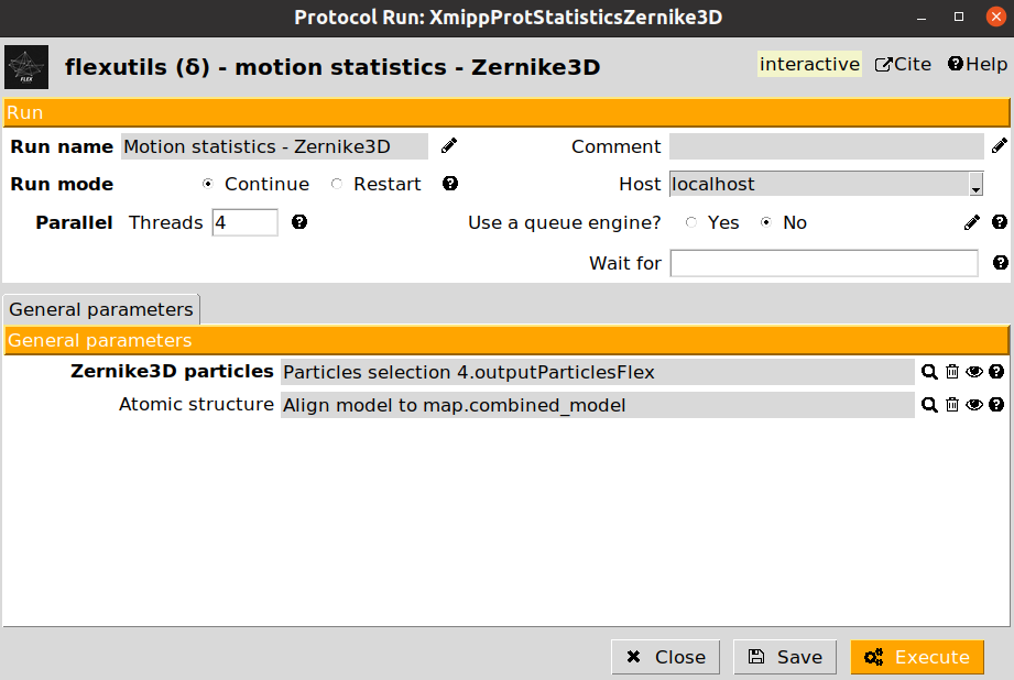
The protocol form includes two different parameters:

• Zernike3D particles: A set of flexibility particles (with Zernike3D information associated) to be analyzed.

• Atomic structure: Optional parameter. if provided, the deformation field could be visualize with either the CryoEM map or an structural model. Otherwise, only the CryoEM map visualization will be available.

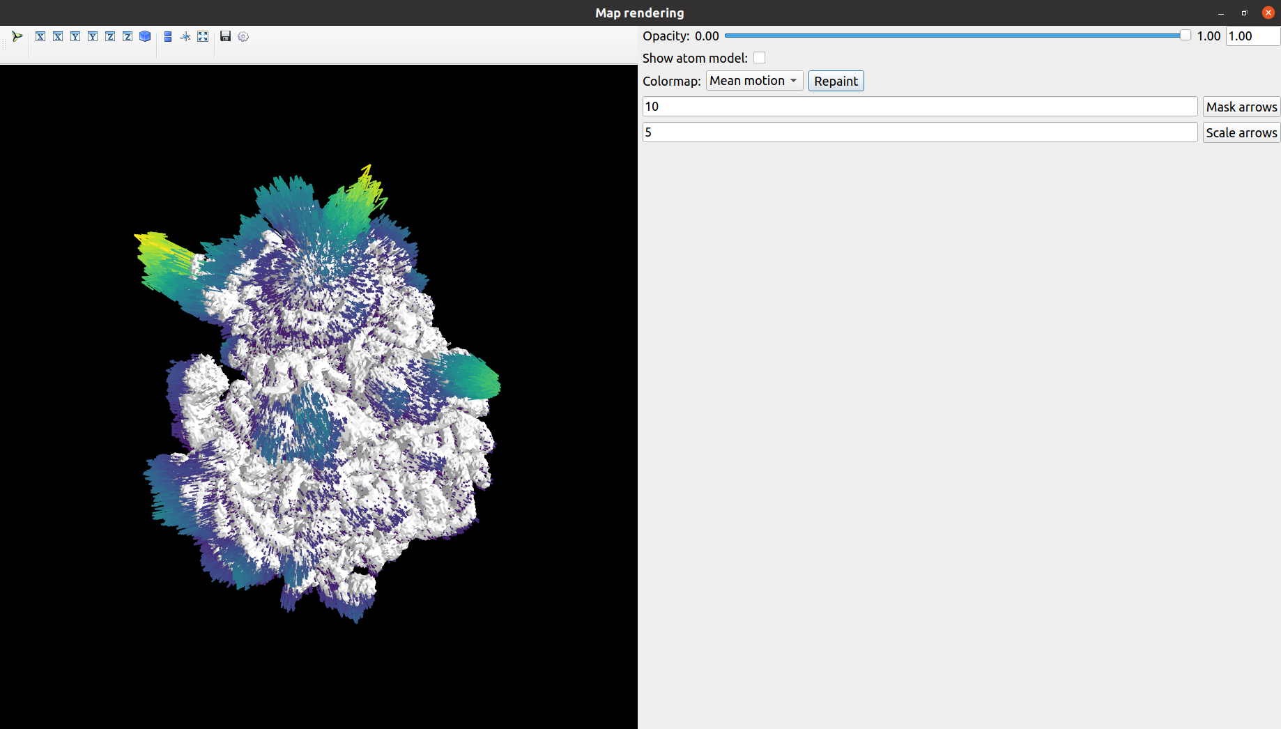
Once the protocol is executed, it will display an interactive visualization displaying the deformation fields together with the CryoEM map or structural model. We provide and example of the window below:

A more in detailed explanation of the viewer interface is available in the following video.

10. Map refinements and ZART

Particles extracted from an interactive conformational space clustering and/or annotation can also be used as part of any standard workflow in Scipion. For example, the extracted particles could be used to refine a given conformation with Relion, CryoSPARC, Xmipp… in order to get a new map able to capture that specific conformational state.

It should be noted that particle refinement quality at this stage could be affected by the number of particles extracted, or the conformational mixture present in the dataset. Nevertheless, even for those cases where the refined map reaches a low resolution, refinements are a good way to validate that the conformational landscapes approximations are the ones expected.

Instead of working with a reduced particle dataset during a refinement, the Flexibility Hub also includes a novel reconstruction algorithm able to correct for an estimated conformational landscape during the reconstruction. In this way, it is possible to increase the resolution of the felxible regions in a map by reducing the motion blur induced by the conformational heterogeneity present in a dataset.

The protocol reconstruct ZART is the responsible for this task. An example of a ZART protocol form is provided below:

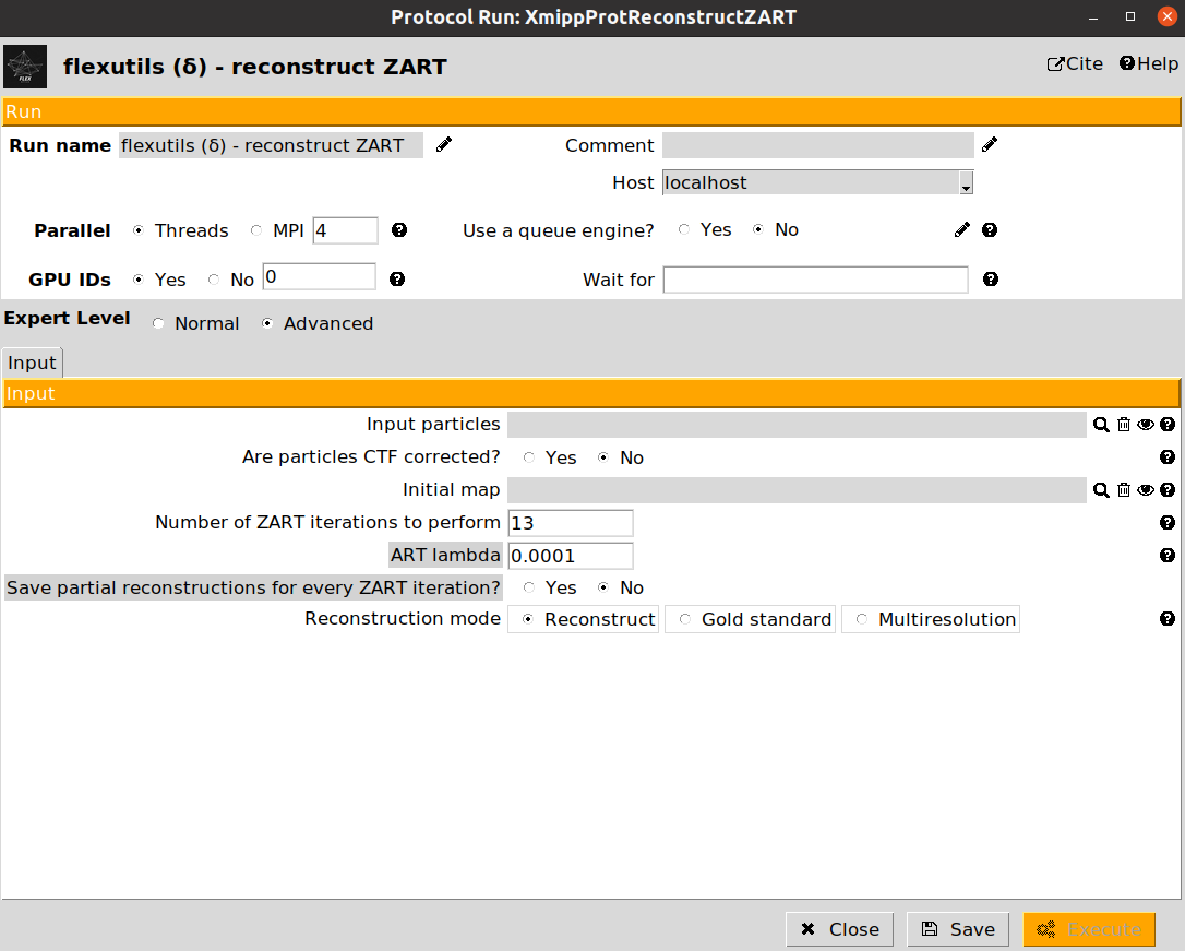
The description of the form parameters is included below:

• Input particles: A set of particles to be reconstructed. They must have angular information stored (CTF is optional).

• Are particles CTF corrected?: Determines whether to correct the CTF during the reconstruction (default) or to skip CTF correction.

• Initial map: If provided, ZART will perform a refinement of this map. Otherwise, a reconstruction is carried out.

• Number of ZART iteration to perform: Number of ART iterations to be done in order to reconstruct a map. We recommend setting a value between 7 and 10.

• ART lambda: Value of the ART regularization to be considered during the reconstruction. If you have a large number of particles (>100k) we recommend decreasing the value to 1e-5.

• Reconstruction mode: Whether to do a standard reconstruction with all the particles, a gold-standard reconstruction of even/odd particles, or a multi-resolution reconstruction.

If the input particles provided have Zernike3D information associated, a new form parameter will be displayed Correct motion blurr artifacts?. If set to yes, ZART will use the estimated conformational landscape information to correct for the conformational heterogeneity in the dataset and improve the reosolution of flexible areas in the macromolecule.

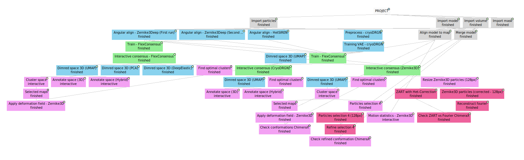
11. Workflow summary

Here finishes the Flexibility Hub Advanced guide!

Below we provide an example of the workflow we have defined along the tutorial. The complete template workflow is available inside the scipion-em-flexutils plugin, inside the templates folder (the path to your template in your system should be : path/to/scipion-em-flexutils/flextuils/templates/advanced_guide.json). To load the template, you can use the following command: scipion3 template path/to/scipion-em-flexutils/flextuils/templates/advanced_guide.json.