MDSPACE Tutorial v1

Introduction

MDSPACE is a method for extracting continuous conformational landscape from cryo-EM particles based on Molecular Dynamics simulations. The purpose of this tutorial is to give a basic introduction to MDSPACE and learn how to create a MDSPACE workflow step by step in Scipion to process a synthetic cryo-EM dataset of Adenylate Kinase (AK).

Prerequisite

ContinousFlex

MDSPACE requires the plugin ContinuousFlex >= 3.3.17 of Scipion 3. Latest version of continuousflex can be obtained from the plugin manager or installed with the following commands:

git clone https://github.com/scipion-em/scipion-em-continuousflex.git

cd scipion-em-continuousflex

git checkout devel

scipion3 installp -p ./ –devel

It is recommended to run the tests related to MDSPACE before starting the tutorial to ensure everything is properly installed :

scipion3 test continuousflex.tests.test_workflow_GENESIS

scipion3 test continuousflex.tests.test_workflow_MDSPACE

ChimeraX

MDSPACE workflow requires ChimeraX plugin of Scipion installed. The plugin can be obtained from the plugin manager or with the following command:

scipion3 installp -p scipion-em-chimera

VMD

It is recommended to have VMD installed on your system for visualization purposes.

Download tutorial data

Start an empty project

To start with this MDSPACE tutorial, open Scipion 3 and create an empty project (see Figure 1). In the new project window, import MDSPACE workflow template by clicking “Others”-> “import workflow template’ -> “continuousflex-MDSPACE” (see Figure 2). The template will ask for input parameters, you can already enter the path to the particle .star file and the pixel size (2.0 A)

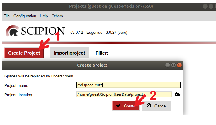
Figure : Creation of a Scipion project. 1) Create an empty project by selecting “Create Project”. 2) Set the project name and location and press “Create”.

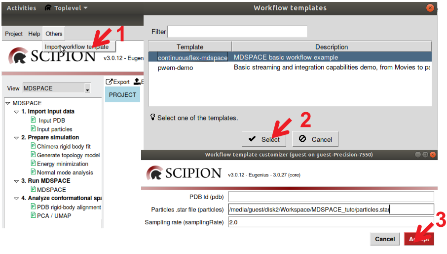
Figure : Import MDSPACE template project. 1) Select “others”-> “Import workflow template” 2) Select MDSPACE template and press “Select” 3) Select the input parameters for the template and press “Accept”

Once the workflow is imported, you can select the view to “MDSPACE” to have a quick access to MDSPACE protocols (see Figure 3)

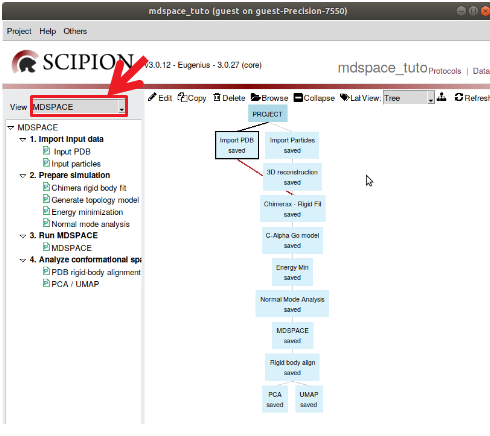
Figure : View of the tree of the MDSPACE template project. Select the view “MDSPACE” to access all the protocols required to run MDSPACE.

Import data

The first protocols to run are the ones that import the data required for MDSPACE into Scipion. The only data required to run MDSPACE are the particles (with the particle pose) and an atomic structure.

Import PDB

Open the protocol “Import PDB”, select the downloaded PDB “AK.pdb” and execute. You can view the structure in ChimeraX by opening the protocol viewer (the button “Analyze Results” in Scipion opens the viewer of a protocol) (See Figure 4).

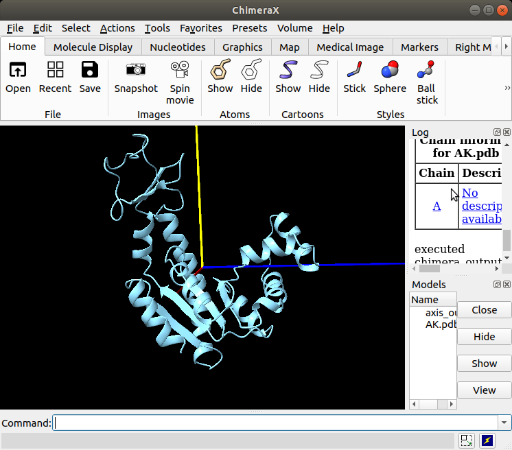
Figure : Imported structure of AK shown in ChimeraX.

Import particles

Open the protocol “Import particles”. Select import from “Relion”, select the downloaded .star file “particles.star” file and execute (Note that scipion-em-relion plugin is required to import data from relion. You can obtain it with scipion3 installp -p scipion-em-relion). Click on “Analyze results” to open the viewer (see Figure 5)

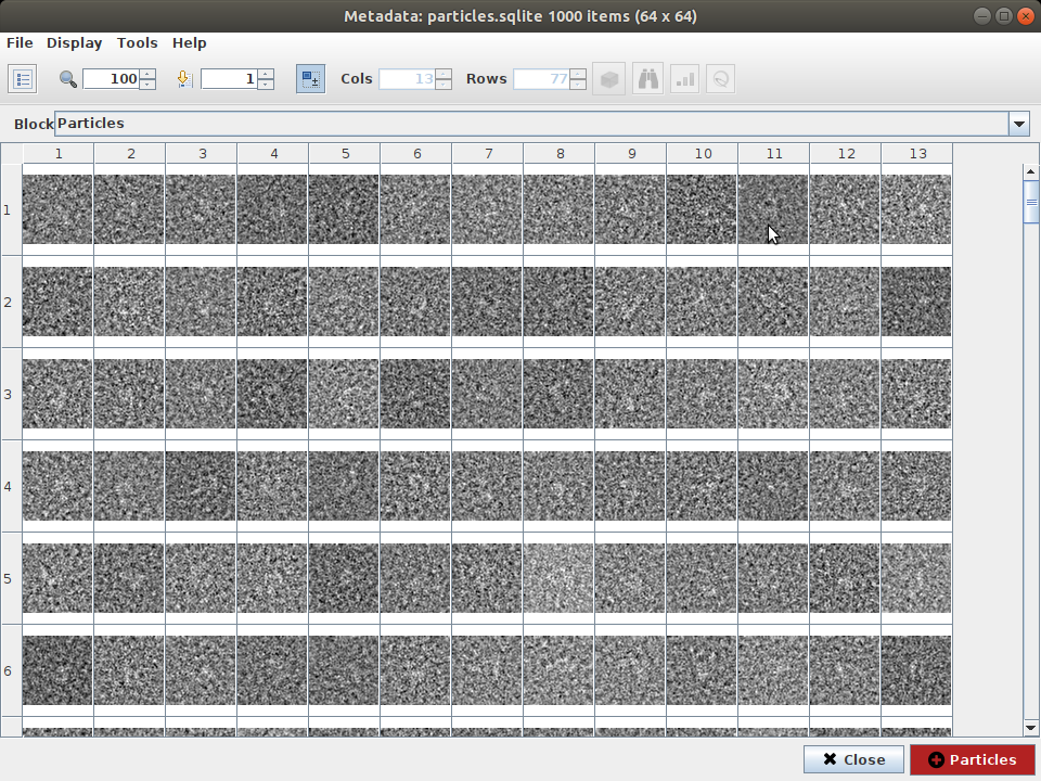
Figure : Imported synthetic particles of AK.

3D reconstruction

To ensure that the particles are imported with the correct particle pose, you can perform a 3D reconstruction of the particles. Execute the protocol “3D reconstruction” and open the EM map into Xmipp/ChimeraX by clicking on “Analyze results”. The 3D reconstruction should match the imported structure.

Prepare simulations

ChimeraX RigidFit

Before running MDSPACE, the imported atomic model must be aligned with the particles in order to optimize the fitting of MDSPACE. Therefore, we need to ensure that the model is aligned with the EM map reconstructed from the particles. For that, run the protocol “ChimeraX RigidFit” with the EM map and the PDB as inputs. By opening ChimeraX, you can see that the model is misaligned with the map. The Figure 4 shows the procedure to align the model with the EM map.

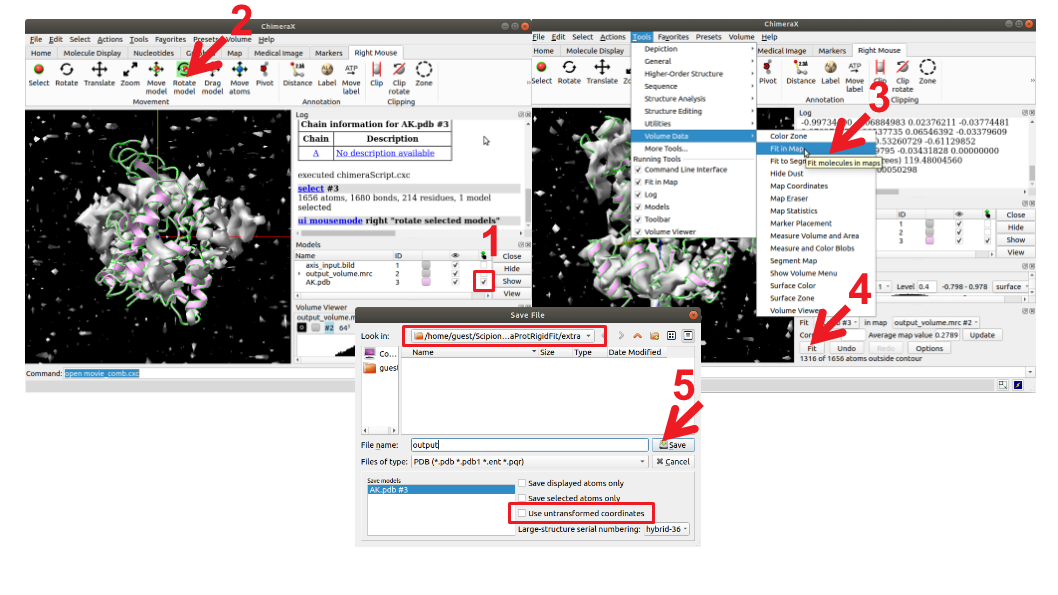
Figure : Rigid body fitting of the atomic model into the EM map with ChimeraX. 1) Select the model you want to move (the atomic model of AK). 2) Select “Right Mouse” -> “Rotate model” or “Move model”, then displace/rotate the model with the right mouse to be close enough of the EM map. 3) Once the model and the map are close enough, you can perform an automatic fitting. Select “Tools” -> “Volume Data” -> “Fit in map”. 4) press “Fit”. 5) Make sure to save the model into the protocol “extra” folder so that Scipion recognize the fitted model. Don’t forget to untick the button “Use untransformed coordinates” to apply the transformation to the model.

C-alpha Go Model

Any MD simulation relies on a forcefield that defines the forces and interactions that will be accounted in the simulation. Many forcefield models exist in MD simulations, that could be all-atoms or coarse-grained. Here we will use a coarse-grained Go-model using carbon alpha atoms only, a Go-like model that simulates the backbone dynamics and largely reduce the computational time of the simulations compare to all-atom simulations such as CHARMM model. Execute the protocol named “C-alpha Go model” and ensure that the output model corresponds to the expected coarse-grained model.

Energy Minimization

The minimization is an important step before running any MD simulation, to ensure that the model is at minimum energy (otherwise, the simulation might get unstable). The protocol for energy minimization uses GENESIS (as well as the protocol for MDSPACE and the other MD simulation tools in ContinuousFlex). GENESIS is a powerful and highly parallelizable MD software that will be use in the backend to perform the MD simulations. The protocol for minimization contains many parameters that could be used to run different type of simulation. Here, you can select the simulation type to “Minimization” and leave all the other parameters to default (See Figure 5).

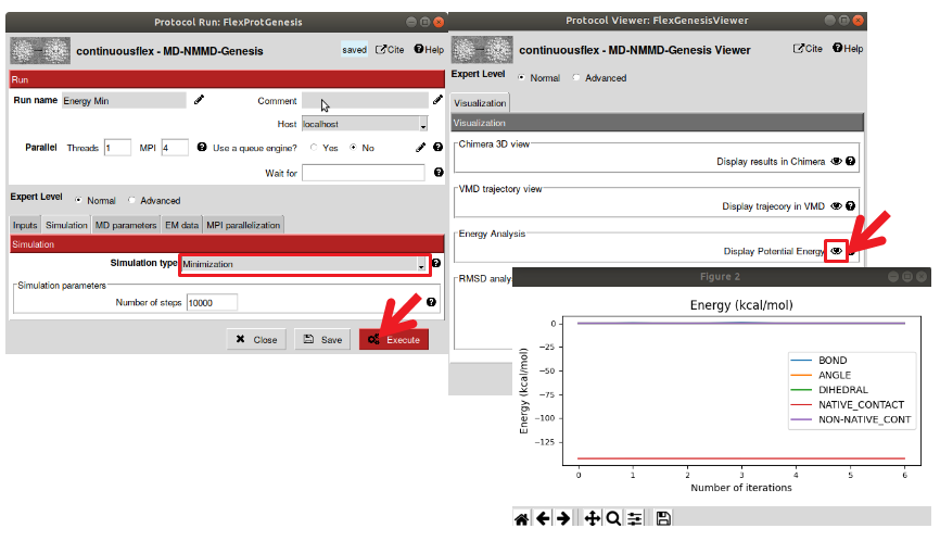
Figure : Perform energy minimization of the model. Open the “Energy Minimization” protocol (FlexProtGenesis) and selection the simulation type to “Minimization” and execute with the default parameters. The viewer displays simulation parameters, select “display potential energy” to view the variation of energy. Here the model was already close to minima therefore the energy remains constant.

Normal Mode Analysis

In MDSPACE, the MD simulations are empowered using normal mode analysis (NMA) through Normal Mode Molecular Dynamics (NMMD). NMA can be used to describe number of flexible states of a structure while having the advantage of being very fast compared to MD simulations. NMA decompose the flexible motions of a structure around an equilibrium with a set of vectors of motions called “normal modes”. NMMD include the most collective normal modes (low-frequency normal modes, that describe global conformational changes) in the MD simulation which boost the motions along the most global conformational changes. To use NMMD, you need to first perform NMA. For that, run the protocol “Normal Mode Analysis” with the default parameters. The NMA viewer allows to observe each computed normal mode in VMD (see Figure 8)

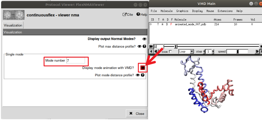
Figure : Display the calculated normal modes. Open the viewer of NMA analysis, then select the normal mode you want to view (modes 1-6 are skipped as they correspond to rigid-body transformations). Select “Display mode animation with VMD” to view the animated motions along one particular mode.

Run MDSPACE

Now that the model is aligned to the particle, energy minimized and that normal modes are calculated, you are ready to run MDSPACE. Open the MDSPACE protocol (see Figure 9).

Parallel Section

The first parameter to define are the “Parallel” section that should be set according to your system configuration (MPI is the number of physical cores and Threads is the number of virtual threads per core).

Inputs

In this section, you define the input of the simulation. In our case, we can restart the previous minimization by selecting “restart previous GENESIS simulation” and select the minimization protocol.

Simulation

In this panel, you define the type of simulation that you want to perform (Energy Minimization, MD simulation, normal mode empowered MD – NMMD, replica exchange MD, etc.). Select “Normal mode molecular dynamics”. A time step of 0.002 ps can be used for this complex but for larger complex, you may need to decrease the time step to 0.001 ps or 0.5 fs to ensure the stability of the simulation. The number of steps here is set to 20000 to obtain 40 ps simulation (20000x0.002 = 40ps), some complex would need longer simulation to reach the full range of variability.

MD parameters

This section defines the parameters used for the MD simulations, you can leave most parameters default, but ensure to decrease the temperature to bellow 100K when using C-Alpha Go model (The C-Alpha Go model overestimate the temperature of the system, so we need to manually decrease it otherwise the simulation will get unstable).

EM data

This section defines the EM data to process with MDSPACE. Select “Images”, and chose the 1000 particles, set the pixel size to 2.0 A² and the projection angles from the image set. The force constant is the most difficult parameter to set. High values will constraint the fitting to the data but tend to overfitting which lead to distortions in the structure. Low values will not constraint the fitting enough and the simulation may not reach the underlying conformational state in the particles. The other fitting parameters can be set to default.

MPI parallelization

This section defines how the simulations are distributed to the available resources. For most local machines, the default parameters will work, you only need to set the number of cores and threads in the “Parallel” section in the top left corner according to your resources. When running on clusters with multiple nodes, it is recommended to set “run on cluster” to efficiently distribute the simulation to each node. If you are using the queuing system of Scipion, you still have to enter all the fields according to your cluster configuration.

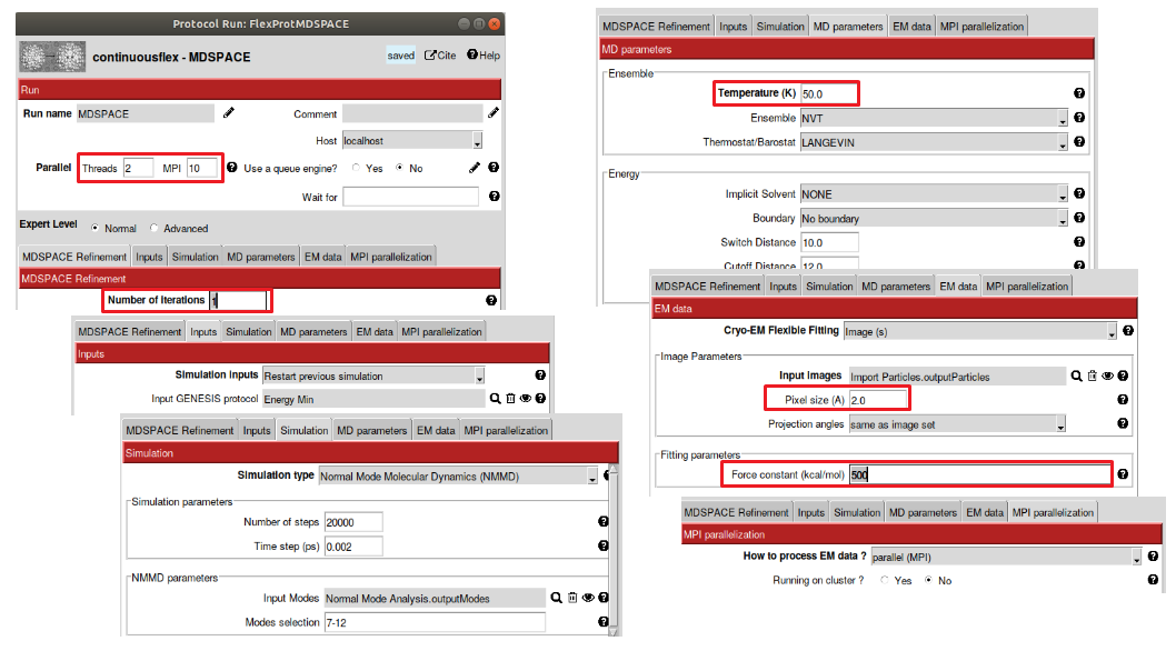
Figure : Protocol for MDSPACE. In the parallel section, select the number of MPI cores and threads according to your configuration. Then select the number of iterations for MDSPACE (here 1 is enough). In the “Simulation” section, select “Normal mode molecular dynamics” and chose the corresponding normal modes. In the “MD parameters”, make sure the temperature is set to low values when using C-alpha Go model for the simulation (<100K). In the “EM data“ section select the particles to fit, don’t forget to select the pixel size to 2.0 A² and the force constant to 500 kcal/mol

Analyze MDSPACE results

MDSPACE viewer

Once MDSPACE execution is completed, you can use the “Analyze Results” button to open the protocol viewer (see Figure 10). This viewer allows to observe the trajectory of each simulation (3D structure, energy, correlation coefficient, RMSD,

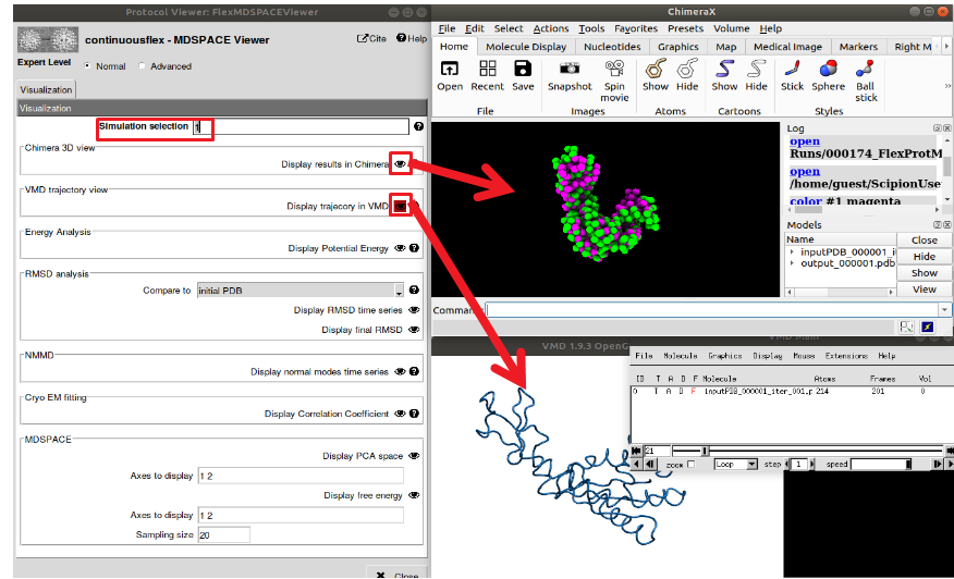
Figure : MDSPACE viewer. The “simulation selection” field determine which simulation will be displayed, you can choose either one simulation (e.g. “1” for the first simulation associated to the first particle”), or a range of simulation (e.g. “1-1000” for all the simulations). The “ChimeraX” viewer shows the initial and final conformations of the simulation and the “VMD” viewer shows the trajectory animation.

Conformational space analysis

To observe the distribution of the conformational space engendered by the models fitted by MDSPACE, you can project the models onto a low-dimensional space using dimension reduction methods such as Principal component analysis (PCA), or Uniform Manifold Approximation and Projection (UMAP). PCA is a well-established method for dimension reduction that relies on a linear decomposition of the motions. UMAP is a more recent technique that allow to extract non-linear feature in the data and sometimes allows a better separation of the different conformational population.

For that, start by running the “Rigid Body Align” protocol. This protocol aligns the output models of MDSPACE to the initial conformation to get rid of rigid-body motions that could be present. Then run the protocol “PCA” and “UMAP”. To observe the conformational space, atomic trajectories and 3D reconstructed trajectories, see Figure 11.

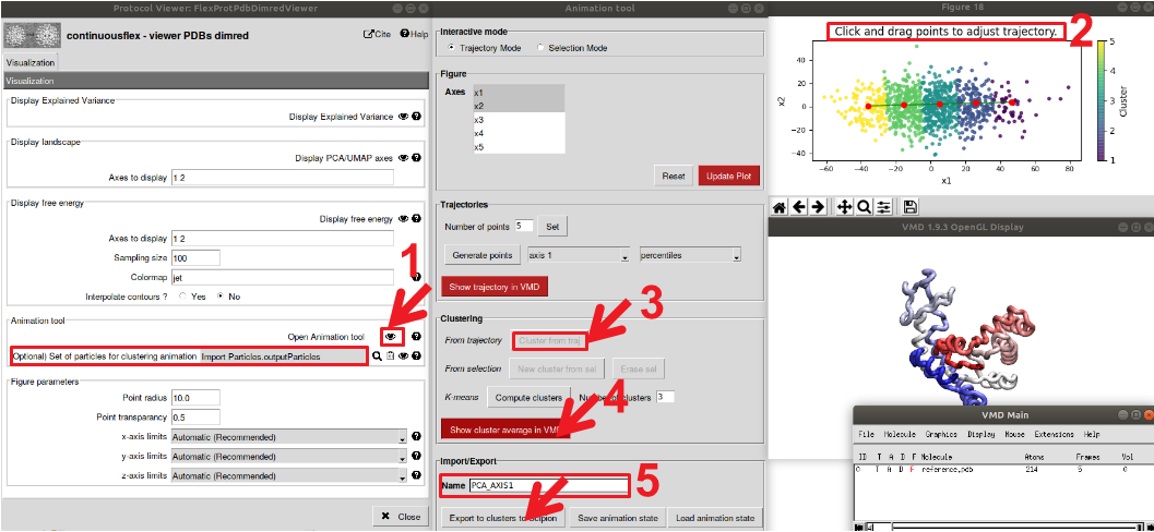
Figure : Analysis of the conformational space determined by MDSPACE using PCA. Open the “viewer PDBs dimred” viewer. 1) open the “Animation Tool”. Two windows will appear, the animation tool and the current conformational space (by default the first 2 PCA axis). 2) Select the “Trajectory Mode” at the top and double click on the conformational space to start placing the trajectory. At this stage you can display the trajectory by clicking on “Show trajectory in VMD” 3) Once all points are placed, select “cluster from traj” to perform clustering of the space based on your trajectory, 4) then display the cluster average in VMD. 5) Finally, you can export the clusters to Scipion. Make sure to give a name to the clusters and to select the particle to which the clusters are apply (in the first window “viewer PDBs dimred”)